- Logistic regression is a type of statistical analysis used to model the relationship between a binary dependent variable and one or more independent variables.
- You can also think of the output as being categorical, with only two possible outcomes.
- Logistic Regressions predict the probability of an event occurring.
Logistic vs Logit Function
This is the Logistic Function. It is a bit complex and it not used as often in models.
\[ p(X) = \frac{e^{\beta_0 + \beta_1x_1 + … + \beta_kx_k}}{1 + e^{\beta_0 + \beta_1x_1 + … + \beta_kx_k}} \]
This is the Logit Function. It is less complex and is used frequently in logistic models.
\[ log(odds) = \beta_0 +\beta_1x_1 + … + \beta_kx_k \]
Logistic Regression Summaries
Below is an example Summary of a dataset:

- Method: MLE (Maximum Likelihood Estimation):
- A function which estimates how likely it is that the model at hand describes the real underlying relationship of the variables.
- The bigger the likelihood function, the higher the probability that our model is correct.
- MLE tries to maximize the likelihood function.
- Log-Likelihood: usually negative. The bigger, the better.
- LL-Null (Log Likelihood Null):
- the log likelihood of a model which has no independent variables.
- This is the constant that we add with the .addConstant() method.
- We often compare the Log-Likelihood of our model with the LL-Null.
- LLR p-value (Log Likelihood Ratio):
- Based on the Log Likelihood and LL-Null.
- It measures if our model is statistically different from the LL-Null, a.k.a. a useless model.
- Pseudo R-squared:
- There is no true R2 measure for logistic regressions.
- There are several propositions. AIC, BIC, McFadden’s R-squared.
- McFadden’s R-squared is what is displayed in the above picture.
- Good Pseudo R-squared values range from 0.2 to 0.4.
- This is good for comparing different variations of the same model. Note that different models will have completely different and incomparable Pseudo R-squares.
Binary Predictors
- We use Binary Predictors in a Logistic Regression the same way we use dummy variables in linear regressions.
- In logistic regression, a binary predictor is an independent variable that takes on only two possible values, typically coded as 0 and 1. Binary predictors are also known as dichotomous variables, because they divide the data into two categories.
- Binary predictors are commonly used in logistic regression to model the effect of a categorical variable on the probability of an event occurring, where the event is represented by a binary dependent variable. For example, a binary predictor could be used to model the effect of gender (male or female) on the probability of developing a certain disease.
Calculating the Accuracy of the Model
- A confusion matrix is a table that is used to evaluate the performance of a logistic regression.
- The confusion matrix is a 2 x 2 matrix that summarizes the number of true positive (TP), true negative (TN), false positive (FP), and false negative (FN) predictions made by the model.
- The four possible outcomes in a binary classification problem are:
- True positive (TP): the model predicts a positive class label, and the actual class label is also positive.
- True negative (TN): the model predicts a negative class label, and the actual class label is also negative.
- False positive (FP): the model predicts a positive class label, but the actual class label is negative.
- False negative (FN): the model predicts a negative class label, but the actual class label is positive.
- Notable equations:
- Accuracy: the proportion of correct predictions made by the model, calculated as (TP + TN) / (TP + TN + FP + FN).
- Precision: the proportion of true positives among all positive predictions made by the model, calculated as TP / (TP + FP).
- Recall (also known as sensitivity or true positive rate): the proportion of true positives among all actual positive cases, calculated as TP / (TP + FN).
- F1 score: a harmonic mean of precision and recall, calculated as 2 * (precision * recall) / (precision + recall).
- Below is some example python code used to create the confusion matrix:

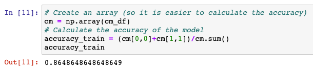
- Now you can easily calculate the Accuracy of this model:
Overfitting and Underfitting
- Overfitting – our training has focused on the particular training set so much, it has “missed the point”. High training accuracy, but outliers cause chaotic graphs. To fix this, split the dataset into a training set and a test set.
- Underfitting – the model has not captured the underlying logic of the data. Low accuracy. Usually a different model is needed.