Descriptive Statistics

Descriptive statistics are numerical measures that summarize and describe the main features of a dataset. They provide a way to understand and interpret the data by presenting it in a meaningful and concise manner.

Population and Sample

• The first step of every statistical analysis you perform is to determine if the data you are dealing with is a population or a sample.
• Population – the collection of all items of interest to our study. Denoted by N. The numbers we gather for a population are called parameters.
• Sample – a subset of the population. Denoted by n. The numbers we gather for a sample are called statistics.
• Samples are less time consuming and less costly to analyze than populations.
• A sample must have both randomness and representativeness for an insight to be precise.
  • Randomness – a random sample is collected when each member of the sample is chosen from the population strictly by chance.
  • Representativeness – a representative sample is a subset of the population that accurately reflects the members of the entire population.

Types of Data and Measurement Levels

We can classify Data in two main ways:

1. Types of Data
   • Categorical – describes categories or groups. Example: car brands, answers to yes/no questions.
   • Numerical – represents numbers.
     • Discrete – can be counted in a finite manner. Example: number of children you want to have, or SAT grades, a number of objects, bank notes, coins.
     • Continuous – infinite and impossible to count. Example: body weight, height, area, distance, time.
2. Measurement Levels
   • Qualitative –
     • Nominal – categories that cannot be ordered, such as car manufacturers, or seasons of the year.
     • Ordinal – consists of groups and categories which follow a strict order. Example: surveys questions that have ranked answers like ‘poor’, ‘fair’, ‘good’, ‘great’, and ‘superior’.
   • Quantitative –
     • Interval – Do not have a true zero. Not as common. Example: temperatures in Celsius and Fahrenheit.
     • Ratio – have a true zero. Examples: number of objects, distance, time, temperature in Kelvin.

Categorical Variables – Visualization Techniques

1. Frequency Distribution Tables
2. Pie Charts
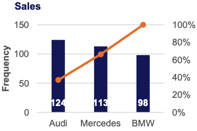
3. Bar Charts
4. Pareto Diagrams – a special kind of bar chart where categories are shown in ascending order of frequency.

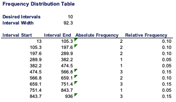
Numerical Variables – Frequency Distribution Table

Frequency Distribution Tables can show either the actual number of observations falling in each range or the percentage of observations. In the latter instance, the distribution is called a relative frequency distribution.

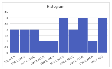
Histograms

A histogram is a graph used to represent the frequency distribution of a few data points of one variable. Histograms often classify data into various “bins” or “range groups” and count how many data points belong to each of those bins.

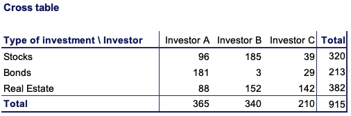
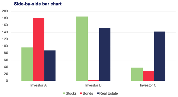
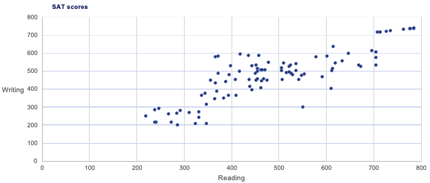
Cross Tables and Scatter Plots

A way to visually represent relationships between two variables.

Categorical Variables

Use Cross Tables to represent Categorical Data.

Side-by-Side bar charts are often used to represent data from Cross Tables.

Numerical Variables

Use a Scatter Plot to represent data that has two numerical variables. Scatter plots usually represent lots of data points.

Mean, Median, and Mode

Known as the three Measures of Central Tendency. Use these together for optimal understanding of a dataset.

Mean

• Also known as the simple average.
• Denoted by a µ in populations and x̄ in samples.
• Is easily affected by outliers. Big negative.
• As a result the mean is not enough to make definite conclusions.

Median

• The middle number in an ordered data set.
• The median is value at position (n + 1) / 2 in the ordered list.
• Median is not affected by outliers.

Mode

• The value that occurs most often.

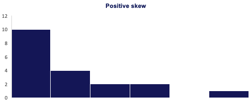
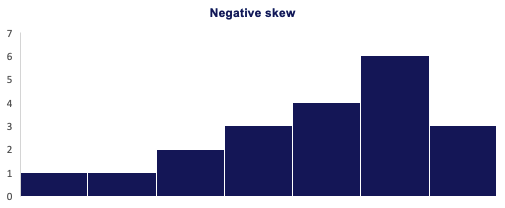
Skewness

• A measure of asymmetry.
• Software is often used to calculate this.
• Skewness indicates if data is concentrated on one side.
• Right (Positive) skewness means that the outliers are to the right (long tail to the right).
• Left (Negative) skewness means that the outliers are to the left.
• Zero skew occurs when the distribution is symmetrical.

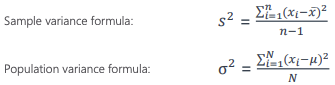
Variance

• Variance measures the dispersion of a set of data points around their mean.
• Variance, Standard Deviation, and Coefficient of Variation are measurements of variability.
• There are different formulas for population data and sample data.

Standard Deviation and Coefficient of Variation

There are different formulas for population data and sample data.

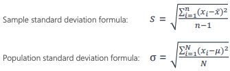
The Coefficient of Variation (CV) also known as Relative Standard Deviation = standard deviation / mean.

Population Formula:

Sample Formula:

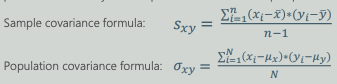
Covariance

• Covariance and the Linear Correlation Coefficient are used to measure the relationship between variables.
• Covariance measures the correlation between two variables.
  • Positive Covariance means the two variables move together.
  • Negative Covariance means the two variables move in opposite directions.
  • 0 Covariance means the variables are independent.
• The drawback of Covariance is that the the range of values is dramatic.
• There are separate formulas for Samples and Populations.

Linear Correlation Coefficient

• Correlation is a measure of the joint variability of two variables.
• Unlike covariance, correlation could be thought of as a standardized measure.
• It takes on values between -1 and 1, thus it is easy for us to interpret the result.
  • A Correlation Coefficient of 1 means the entire variability of one variable is explained bo the other variable.
  • A Correlation Coefficient of 0 means the variables are absolutely independent.
• The linear Correlation Coefficient has the following basic equation:

There are different formulas for Samples and Populations:

Statistics Glossary

Descriptive Statistics Cheat Sheet