Neural Networks

Layers in Neural Networks

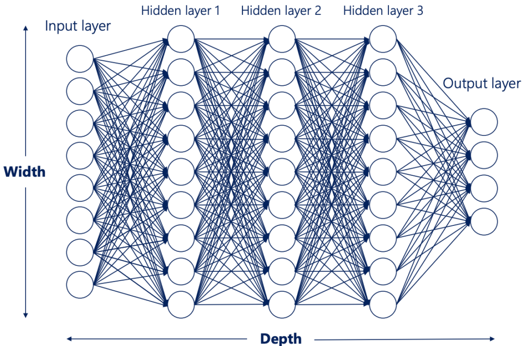
In a neural network, a layer refers to a group of interconnected nodes, also known as neurons or units, that process and transform the input data. Layers are organized in a sequential manner, with each layer receiving input from the previous layer and passing its output to the next layer. The arrangement and number of layers in a neural network architecture define its depth and complexity.

Neural networks typically consist of multiple layers, each serving a specific purpose in the overall computation. The three main types of layers in a neural network are:

1. Input Layer:
   • The input layer is responsible for receiving the initial input data and passing it to the subsequent layers.
   • The number of nodes in the input layer corresponds to the number of features or dimensions in the input data.
2. Hidden Layers:
   • Hidden layers are the intermediate layers between the input and output layers.
   • They perform complex computations by applying weighted transformations to the input data, using activation functions to introduce non-linearities.
   • Deep neural networks have multiple hidden layers, which allow for hierarchical representations and the extraction of higher-level features.
3. Output Layer:
   • The output layer is the final layer of a neural network, which produces the network’s predicted outputs or class probabilities.
   • The number of nodes in the output layer depends on the nature of the task. For example, in a binary classification problem, the output layer may have a single node representing the probability of belonging to the positive class. In multi-class classification, the number of nodes corresponds to the number of classes.

The arrangement and configuration of layers in a neural network architecture, known as the network topology, can vary depending on the problem at hand. Different architectures, such as feedforward neural networks, convolutional neural networks (CNNs), or recurrent neural networks (RNNs), have specific layer configurations tailored to specific tasks, such as image classification, natural language processing, or time series analysis.

Width and Depth of a NN

• The width of a layer is the number of units in that layer
• The width of the net is equal to the number of layers or the number of hidden layers.
• The depth of the net is the number of units of the biggest layer. The term has different definitions. More often than not, we are interested in the number of hidden layers (as there are always input and output layers).
• The width and the depth of the net are called hyperparameters. They are values we manually chose when creating the net.

Selecting the Width of a Neural Network

There are many rule-of-thumb methods for determining the correct number of neurons to use in the hidden layers, such as the following:

• The number of hidden neurons should be between the size of the input layer and the size of the output layer.
• The number of hidden neurons should be 2/3 the size of the input layer, plus the size of the output layer.
• The number of hidden neurons should be less than twice the size of the input layer.

Moreover, the number of neurons and number layers required for the hidden layer also depends upon training cases, amount of outliers, the complexity of, data that is to be learned, and the type of activation functions used.

Most of the problems can be solved by using a single hidden layer with the number of neurons equal to the mean of the input and output layer. If less number of neurons is chosen it will lead to underfitting and high statistical bias. Whereas if we choose too many neurons it may lead to overfitting, high variance, and increases the time it takes to train the network.

Pruning

Pruning can be used to optimize the number of neurons in the hidden and increases computational and resolution performances. It trims the neurons during training, by identifying those which have no impact on the performance of the network. It can also be identified by checking the weights of the neurons, weights that are close to zero have relatively less importance. In pruning such nodes are removed.

Non-Linearities and their Purpose

Each line on the above diagram represents a linear combination with an associated weight and bias, followed by a non-linear element. This allows us to model arbitrary functions.

In order to have deep nets and find complex relationships through arbitrary functions, we need non-linearities.

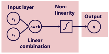
Activation Functions (Transfer Functions)

Activation function are the non-linearities that we discussed above.

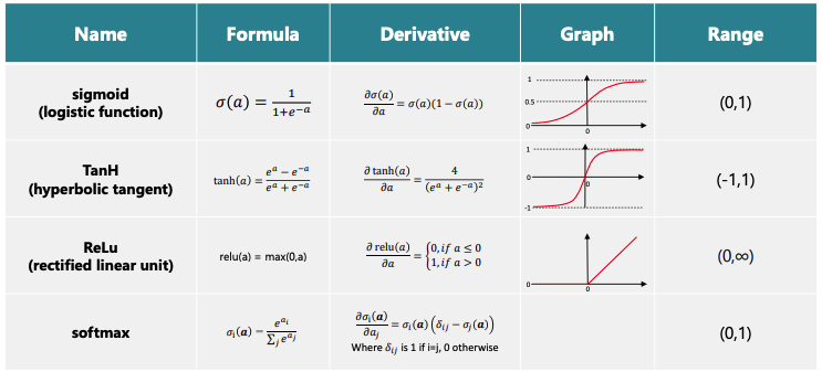
Note that softmax calculates differently than the other Activation Functions. It calculates using information from all elements, whereas the other Activation Functions calculate stepwise. softmax is often used in the output layer. Also note that the sum of the outputs of softmax equals 1.

• Note that softmax calculates differently than the other Activation Functions. It calculates using information from all elements, whereas the other Activation Functions calculate stepwise.
• Softmax is often used in the output layer.
• Also note that the sum of the outputs of softmax equals 1, and is a probability distribution.

Backpropagation

Backpropagation, short for “backward propagation of errors,” is a key algorithm used in training neural networks. It enables the network to learn from labeled training data by iteratively adjusting the weights and biases of the network’s connections.

Here’s a step-by-step explanation of the backpropagation algorithm:

1. Forward Pass:
   • During the forward pass, input data is fed into the neural network, and activations are calculated layer by layer, propagating from the input layer to the output layer.
   • Each layer applies a weighted sum of inputs, adds a bias term, and applies an activation function to produce the output or activation values.
2. Calculate Error:
   • Once the forward pass is complete and the network produces output, the error between the predicted output and the actual output is calculated using an appropriate loss function.
   • The loss function measures the discrepancy between the predicted and actual values and provides a measure of the network’s performance.
3. Backward Pass:
   • The backward pass is where the actual backpropagation occurs. It involves propagating the error from the output layer back to the previous layers to update the weights and biases.
   • Starting from the output layer, the derivative of the loss function with respect to the activations is computed.
   • The derivative is then used to calculate the gradients of the weights and biases in each layer using the chain rule.
4. Weight and Bias Updates:
   • The gradients obtained in the backward pass are used to update the weights and biases in each layer of the neural network.
   • The learning rate, a hyperparameter, determines the size of the update step. A higher learning rate leads to larger parameter updates, while a lower learning rate results in smaller updates.
   • The weights and biases are adjusted by subtracting the learning rate multiplied by the corresponding gradients.
5. Repeat the Process:
   • The forward and backward passes are repeated for multiple iterations or epochs to refine the network’s weights and biases.
   • The process of forward pass, error calculation, backward pass, and weight updates is iterated until a stopping criterion is met, such as reaching a maximum number of iterations or achieving satisfactory performance.

By iteratively adjusting the weights and biases based on the calculated gradients, backpropagation allows the neural network to learn from the training data and improve its performance over time. The algorithm computes the gradients layer by layer, efficiently propagating the errors back through the network.

It’s worth noting that backpropagation is typically used in conjunction with optimization algorithms such as gradient descent to find the optimal values for the network’s parameters. The combination of backpropagation and optimization helps neural networks converge towards a minimum of the loss function and achieve better performance on the given task.

Convolutional Neural Networks (CNNs)

Convolutional Neural Networks (CNNs) are a specialized type of neural network designed to process and analyze data with a grid-like structure, such as images or time series data. CNNs have been highly successful in various computer vision tasks, including image classification, object detection, and image segmentation. They are inspired by the organization of the visual cortex in the human brain.

Here’s a description of the key components and operations in a typical CNN:

1. Convolutional Layers:
   • Convolutional layers are the core building blocks of CNNs. They consist of multiple learnable filters or kernels that slide over the input data, extracting local features through convolution operations.
   • Each filter detects specific patterns or features, such as edges, textures, or shapes, by computing element-wise multiplications and summations.
   • Convolutional layers are responsible for automatically learning hierarchical representations of the input data.
2. Pooling Layers:
   • Pooling layers are often inserted between convolutional layers to reduce the spatial dimensionality of the feature maps.
   • Common pooling operations include max pooling and average pooling, which downsample the input by taking the maximum or average value in a local neighborhood.
   • Pooling layers help reduce the computational complexity of the network, introduce spatial invariance, and enhance the network’s ability to capture relevant features.
3. Activation Functions:
   • Activation functions introduce non-linearities into the network, enabling CNNs to learn complex mappings between the input data and the desired outputs.
   • Common activation functions used in CNNs include Rectified Linear Unit (ReLU), sigmoid, and hyperbolic tangent (tanh).
   • ReLU is widely used due to its computational efficiency and ability to mitigate the vanishing gradient problem.
4. Fully Connected Layers:
   • Fully connected layers, also known as dense layers, are traditional neural network layers where each neuron is connected to every neuron in the previous layer.
   • Fully connected layers are typically placed towards the end of the CNN architecture and are responsible for combining the extracted features and making final predictions.
   • The output of the last fully connected layer is often passed through a softmax activation function to obtain probability distributions over different classes.
5. Backpropagation and Training:
   • CNNs are trained using backpropagation, where the gradients of the loss function with respect to the network parameters are computed and used to update the weights through optimization algorithms like Gradient Descent.
   • Training data is usually fed into the network in batches to improve efficiency and generalization.

Recurrent Neural Networks (RNNs)

Recurrent Neural Networks (RNNs) are a type of neural network architecture designed to process sequential data by capturing and utilizing information from previous steps. RNNs are widely used in natural language processing, speech recognition, time series analysis, and other tasks involving sequential or temporal data.

Here’s an overview of the key components and operations in a typical RNN:

1. Recurrent Connections:
   • The distinguishing feature of RNNs is the presence of recurrent connections that allow information to flow from one step to the next within the sequence.
   • These connections create a feedback loop, where the output at each step serves as an input for the next step, enabling the network to maintain memory and consider context from previous steps.
2. Hidden State:
   • RNNs have a hidden state vector that acts as a memory or representation of the information seen so far in the sequence.
   • The hidden state at each step is updated based on the current input and the previous hidden state, capturing the sequential dependencies in the data.
   • The hidden state carries information from earlier steps to later steps and serves as a summary of the sequence up to that point.
3. Activation Function:
   • RNNs apply an activation function to transform the input and hidden state at each step, introducing non-linearities and enabling the network to model complex relationships.
   • Common activation functions in RNNs include sigmoid, tanh, and ReLU.
4. Training and Backpropagation Through Time (BPTT):
   • RNNs are trained using backpropagation through time, an extension of standard backpropagation.
   • BPTT involves unfolding the recurrent connections over time, treating the network as a deep feedforward neural network with shared weights, and propagating errors through each unfolded step.
   • The gradients are accumulated and used to update the network parameters through optimization algorithms like Gradient Descent.
5. Long Short-Term Memory (LSTM) and Gated Recurrent Unit (GRU):
   • To address the vanishing gradient problem and capture long-term dependencies, advanced RNN variants such as Long Short-Term Memory (LSTM) and Gated Recurrent Unit (GRU) have been introduced.
   • LSTM and GRU have additional gates and memory cells that control the flow of information, allowing RNNs to better capture and preserve important information over longer sequences.

RNNs excel at handling sequential data because they can learn to model dependencies and context over time. They can process variable-length sequences and make predictions at each step. However, standard RNNs may struggle with long-term dependencies due to the vanishing gradient problem. LSTM and GRU architectures were developed to address this limitation by providing mechanisms to selectively store and update information.

In practice, RNNs can be stacked to form deeper networks, and bidirectional variants can process sequences in both forward and backward directions. These extensions enhance the model’s ability to capture complex patterns and improve performance in various tasks that involve sequential data.

Backpropagation

Neural Networks Cheat Sheet