SELECT, FROM, WHERE, OR, AND, and ‘like’ Statements
The SELECT Statement
Select all columns from the database named employees:

Select Specific columns from the database, employees:

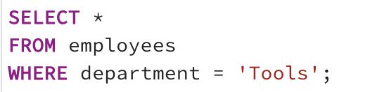
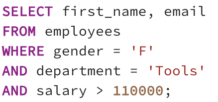
The WHERE Statement
Select all rows where the department is ‘Tools’:
The ‘like’ Statement
Select rows where to department contains the consecutive characters ‘To’:

Select rows where the department name starts with ‘T’ and contains ‘oo’:

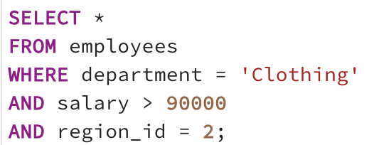
OR and AND Statements


IN, NOT IN, IS NULL, and BETWEEN Statements
IN statements allow you to select several items at once:

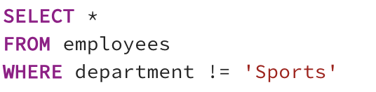
Three ways to invert a selection of data:


Searching for NULL values:

Filtering NULL values:


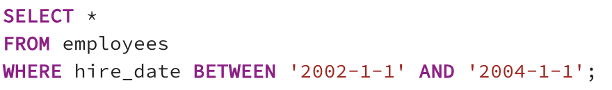
Use BETWEEN to look for a range of values. This is inclusive:

Combine These Words


ORDER BY, LIMIT, DISTINCT and Renaming Columns
ORDER the database BY a column:

ORDER the list in descending order:

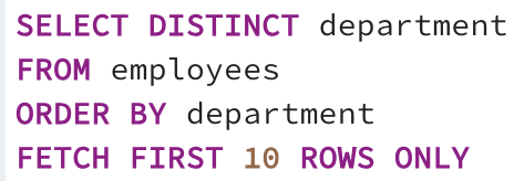
Show unique items from a column:

Show unique items from a column in ORDER:

Two ways to show the first 10 unique items in a column:

Rename a column:

Rename a column with spaces:

Using Functions
UPPER(), LOWER(), LENGTH(), TRIM() + Boolean Expressions & Concatenation
Make a column of data uppercase or lowercase:


Show the length of each cell of data in a column:

Trim spaces from data:

Show the length of the trimmed data:

Show data from two rows concatenated:

Add a space in the title of a new concatenated column:

Also, show true/false for each employees making more than $140,000:

Name this new column ‘wealthy’:

See if a value is contained in data. This returns ‘true’:

This returns ‘false’:

Return true/false for each row of data in departments if they contain ‘oth’:

String Functions: SUBSTRING(), REPLACE(), POSITION() and COALESCE()
Start with some test data:

Select data starting at the 1st position, for 4 characters. ‘This’ will be returned:

Return everything starting at the 9th character:

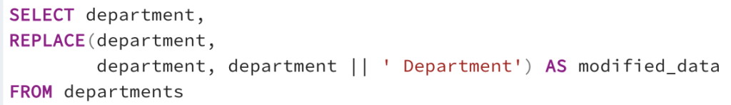
Replace text in data, and save it to a new column. In this case, the ‘Clothing’ and ‘Childrens Clothing’ departments are changed to “Attire’ and ‘Childrens Attire’:

A new column is created, and each department has the word “Department’ added to the end of it.
Select text from each email starting at the ‘@’ symbol:

Select text from each email after the ‘@’ symbol:

Create a new column, and replace NULL emails with the text ‘None’:

Grouping Functions: MIN(), MAX(), SUM(), AVG(), COUNT()


AVG yields a results with many decimal places. ROUND your result for better appearance:


This is an easy way to COUNT the number entries in a table:


Grouping Data and Computing Aggregates
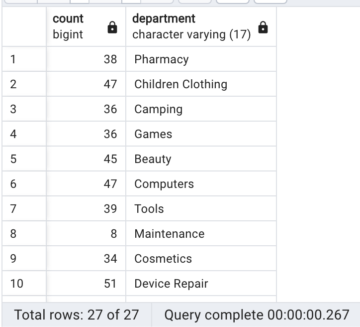
Below we count the number of employees in each department.

Here is the output for this query:

GROUP BY and HAVING Clauses
List the headcount of each department.Note that only a column of head counts is shown here.

Show departments and the head count for each department:

Output for this Query:
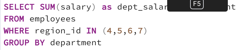
Show the sum of departmental salaries and department names:

Show the sum of departmental salaries where region_id’s are 4, 5, 6, or 7, and display department names:
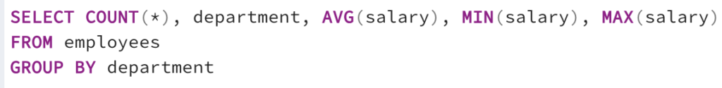
Show the headcount, department name, average salary, minimum salary, maximum salary for each department.
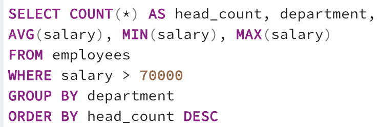
Same as above, but order departments in descending order:

Same as above, but only include people with salaries above $70k:
Create separate columns for gender head count for each department:
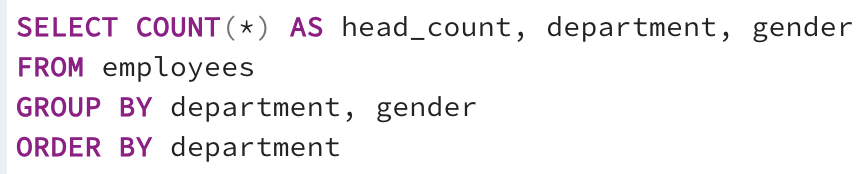
Output from this query:

Use the HAVING command to compare aggregated data:

More Examples
Show a list of first names in the company, and which first names are most common.
Show only the first names that occur more than once in the company.
See which domain names are most common among employee email addresses:
Show min, max, and average salaries for men and women in each region:
Write a query that displays only the state with the largest amount of fruit supply:

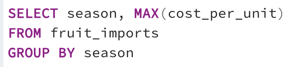
Write a query that returns the most expensive cost_per_unit of every season. The query should display 2 columns, the season and the cost_per_unit:
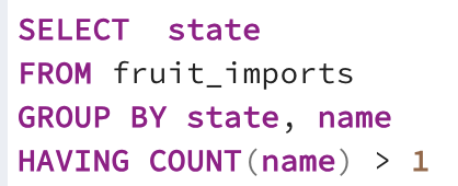
Write a query that returns the state that has more than 1 import of the same fruit:
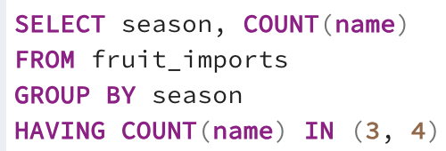
Write a query that returns the seasons that produce either 3 fruits or 4 fruits:
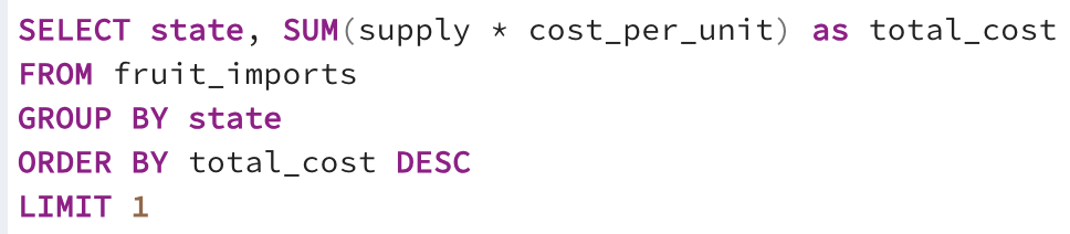
Write a query that takes into consideration the supply and cost_per_unit columns for determining the total cost and returns the most expensive state with the total cost:
Using Subqueries and Aliases
Select fist_name, last_name, and the entire table again:

Select a column from a specific table:


Use Aliases to rename tables:

Subqueries in WHERE and FROM Clauses
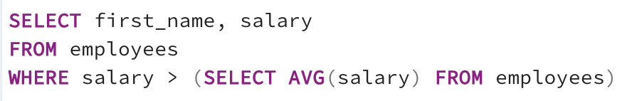
A Subquery in a WHERE Clause:

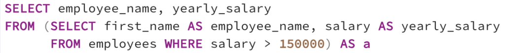
A Subquery in a FROM Clause. Note that the following three queries produce the same result:


The following three queries all produce the same result:

Subqueries Examples
Select all employees who work in the Electronics Division:

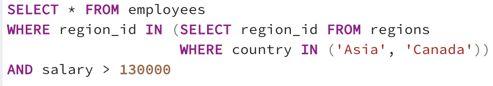
Select all employees who work in Asia or Canada, AND make more than $130,000:
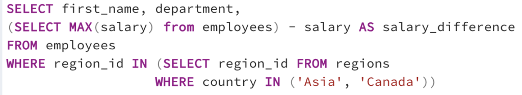
Show the first name, department, and the salary difference from the highest paid employee for those employees in Asia and Canada:
Subqueries with ANY and ALL Operators
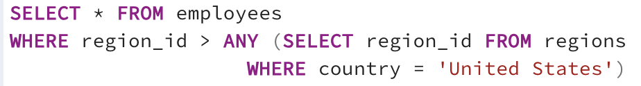
Select all employees working in the United States:

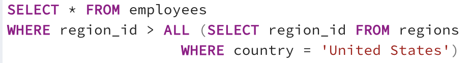
Select all employees whose region_id is greater than ALL of the United States region_id’s. This is not typically used:
Select all employees whose region_id is greater than ANY of the United States region_id’s:
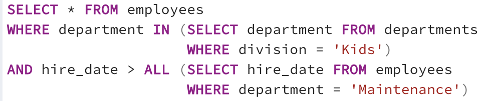
Select all employees who work in the Kids Division, and who have been hired more recently than anyone in the Maintenance department:
Find the most common salary among employees. If there is a tie for the most common salary, return the highest of those salaries:

CREATE and DROP Tables + More Exercises
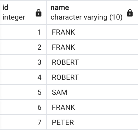
This table will be used in the next exercise:
This table is created with this command:

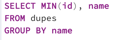
Show the unique names from the table, and the smallest id associated with that name:
Delete the table:

Two ways to determine the average company salary excluding the lowest and highest salary:


Subquery Exercises
These exercises will use these tables:

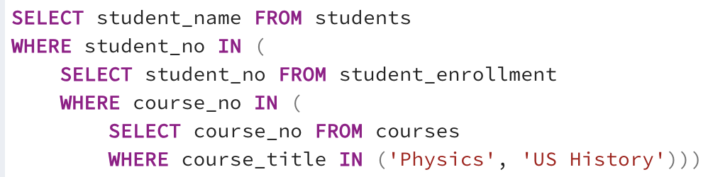
Using subqueries only, write a SQL statement that returns the names of those students that are taking the courses Physics and US History:
Using subqueries only, write a query that returns the name of the student that is taking the highest number of courses:

Write a query to find the student that is the oldest. You are not allowed to use LIMIT or the ORDER BY clause to solve this problem:

Conditional Expressions Using the CASE Clause
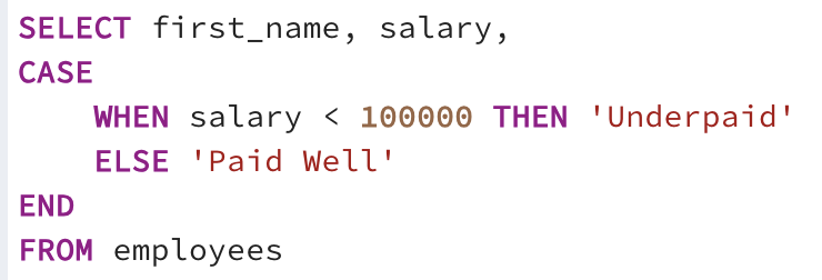
Create a new column that adds an entry of Underpaid or Paid Well, depending on employee income:

Another way to write this:
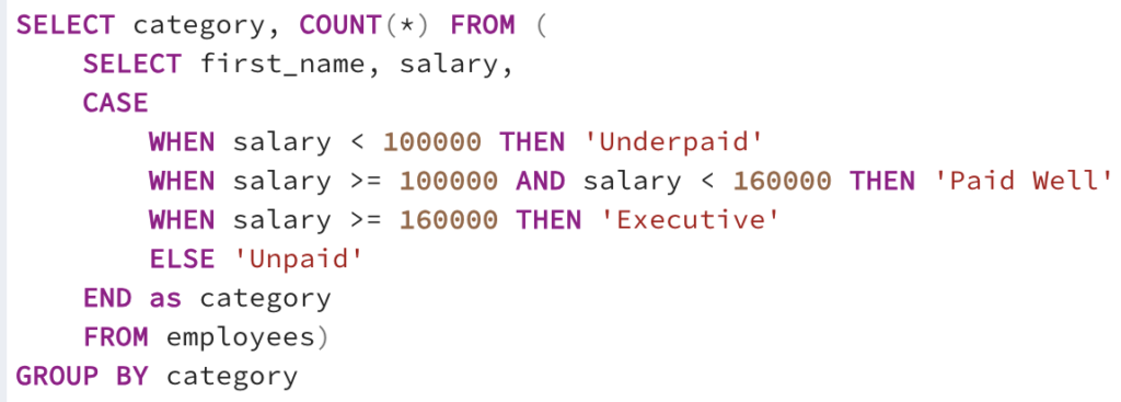
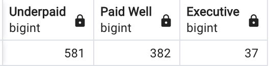
COUNT the CASES below and display them in a table:
This is the resulting table:

Convert rows to columns and columns to rows for this table:

This is the resulting table:
Transposing Data using the CASE Clause
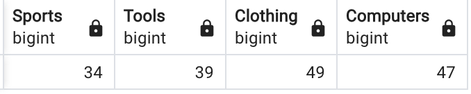
Show columns displaying employee populations for the Sports, Tolls, Clothing, and Computer departments:

The resulting table:
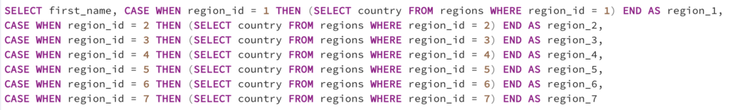
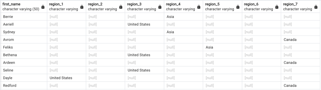
Show a table with employee first names, and seven columns, each representing a region_id. Fill in the continent where that employee works in the appropriate column:
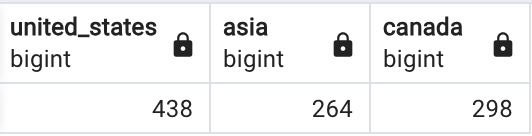
Use the above code to create a column for each continent, followed by the employee population in that continent:

CASE and Transposing Exercises
These exercises will use this table named fruit_imports:
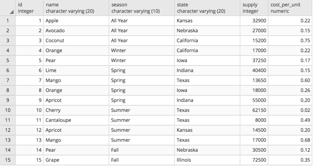
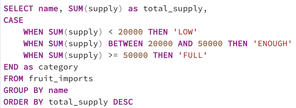
Write a query that displays 3 columns. The query should display the fruit and it’s total supply along with a category of either LOW, ENOUGH or FULL. Low category means that the total supply of the fruit is less than 20,000. The enough category means that the total supply is between 20,000 and 50,000. If the total supply is greater than 50,000 then that fruit falls in the full category:
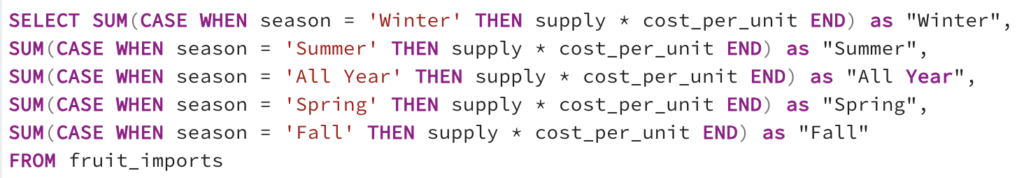
Taking into consideration the supply column and the cost_per_unit column, you should be able to tabulate the total cost to import fruits by each season. The result will look something like this:
“Winter” “10072.50”
“Summer” “19623.00”
“All Year” “22688.00”
“Spring” “29930.00”
“Fall” “29035.00”
Write a query that would transpose this data so that the seasons become columns and the total cost for each season fills the first row?
Advanced Query Techniques Using Correlated Subqueries
This is an example of a Subquery:
Correlated Subqueries are a way to link data form the inner subquery, and the outer query. Note that the inner correlated subquery runs through completion for each iteration of the outer query. This can be processor-heavy.
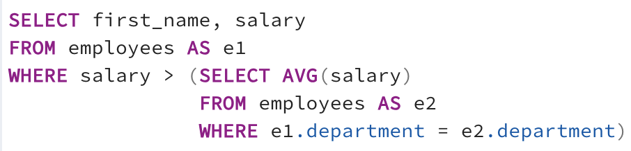
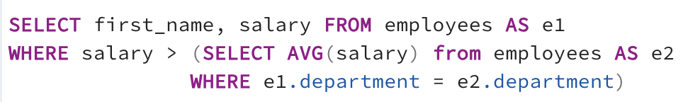
Below, the department columns of the employee tables are correlated. This query displays employee first name, and salary for those employees whose salary is larger than their department’s average salary:
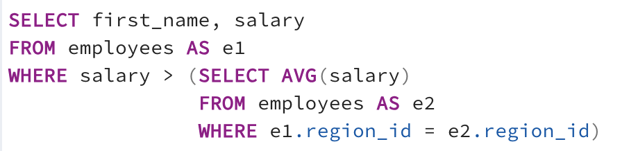
Likewise, this query displays employee first name, and salary for those employees whose salary is larger than their region’s average salary:
Display the first name, salary, department, and average department salary for each employee:

Show a column of department names that have more than 38 employees. Note that this could be more easily accomplished using COUNT(*), WHERE, and a GROUP BY department:

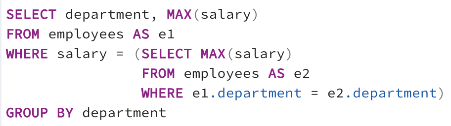
Display each department and the maximum salary from that department:
A better way to accomplish this task. Using the departments table allows for fewer repetitions of calculations during the query:

Correlated Subquery Exercises
Create this table using what you have learned so far:
This code will create the table:

Now show the lowest and highest salary for males and females in each department:
This is the resulting table:

Introducing Table Joins
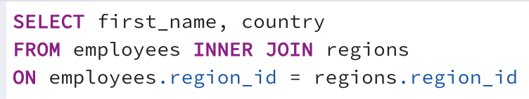
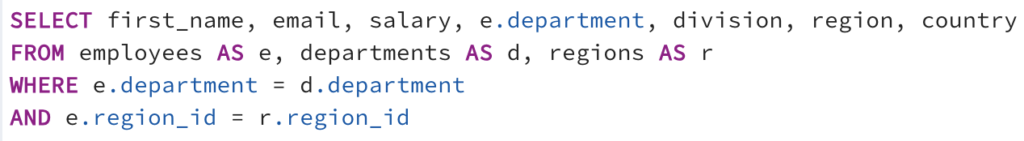
Tables can be Joined by a common column of data. Below, the employees and regions table are joined to display the first name and country of each employee:

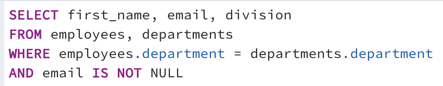
Show the name, email, and division for each employees, only if their email is not NULL:
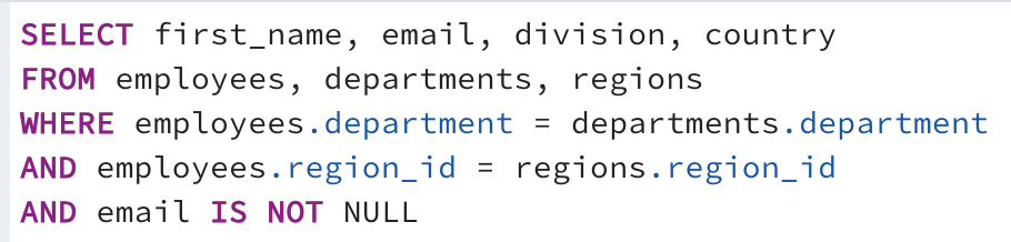
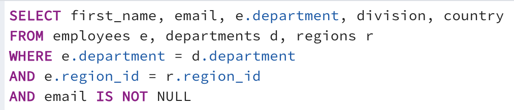
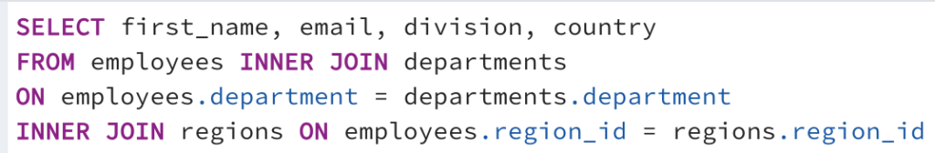
Join three tables. Show the name, email, division, and country, only if their email is not NULL:
To select a column of data that exists in more than one table, name the source table as below:

Table names can have aliases to make notation cleaner:
INNER and OUTER Joins
Show the name and country of each employee by joining the employees and regions tables through the region_id columns:
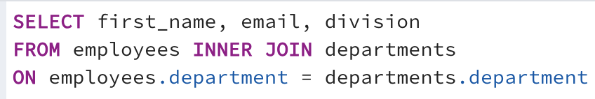
Likewise, show name, email, and division for each employee by joining the employees and departments tables through the department columns:
Below, three tables are joined:
This shows two columns of departments that are common to both department columns. In this case, that is 23 department names:

This shows two columns of departments that are common to both department columns, AND includes all departments from the LEFT (employees) table. This creates a table with 27 rows.

This shows two columns of departments that are common to both department columns, AND includes all departments from the RIGHT (departments) table. This creates a table with 24 rows.

Show only the departments that are unique to the employees table:

Using UNION, UNION ALL and EXCEPT Clauses
Show a column of all the unique department names from the employees and departments tables:

Show a column of ALL department entries from the employees and departments tables:

Show the department names that are in the employees table, but not in the departments table. This is also called MINUS in other query languages:

Show the population of each department, followed by the TOTAL company population:

Cartesian Product with the CROSS JOIN
A Cartesian Product or CROSS JOIN repeats each row in the first table for each row in the second column.
Below, the employees table has 1,000 rows, and the departments table has 24 rows. The resulting table below will have 24,000 rows:

This is a shorthand way to write this CROSS JOIN:

To CROSS JOIN the same table, use aliases to avoid errors:

More than two tables can be joined. Below, a table with 1,000 x 1,000 x 24 = 24,000,000 rows is created.

Joins and Subquery Exercises
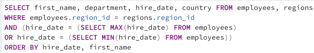
Show the name, department, hire date, and country for the first hire, and the most recent hire:
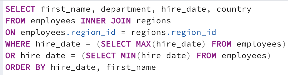
Another way to write this:
Show the sum of the salaries for new hires starting 90 days before their hire date:

The resulting table looks like this:

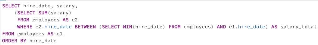
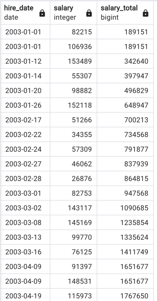
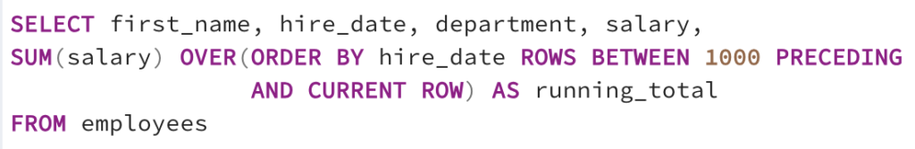
For something a bit easier to grasp, this example shows the running total of annual salaries by hire date:
This is the resulting table:
Creating Views vs. Inline Views
A View is a virtual table based on an existing query. Views can be useful when you need to re-use a complicated query repeatedly. Note that data cannot be added or deleted from a View.
Below we have a query we would like to make a View.
To make it a View, just add the CREATE VIEW line:

Now the information in this View can be accessed like a table. In other words, the query above, and the query below will show the same information:

Inline Views are simply a subquery in the FROM section of a query:

ADVANCED Problems using Joins, Grouping and Subqueries
Use the tables students, courses, student_enrollment, professors, and teach for these exercises.
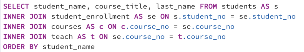
Write a query that shows the student’s name, the courses the student is taking and the professors that teach that course:

Another way to code this:
Above you discovered why there is repeating data. How can we eliminate this redundancy? Let’s say we only care to see a single professor teaching a course and we don’t care for all the other professors that teach the particular course. Write a query that will accomplish this so that every record is distinct. HINT: Using the DISTINCT keyword will not help. 🙂

In the video lectures, we’ve been discussing the employees table and the departments table. Considering those tables, write a query that returns employees whose salary is above average for their given department.
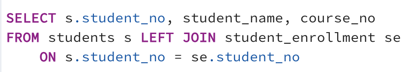
Write a query that returns ALL of the students as well as any courses they may or may not be taking.
Window Functions using the OVER() Clause
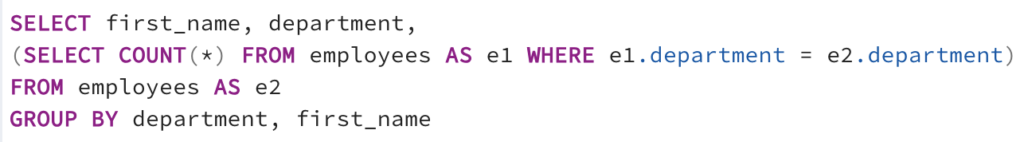
Say you want to show the department headcount in a column along with other employee data. So far, we have had to use a Correlated Subquery like below:
There is a way to use the OVER() clause which is less processor heavy. The following query shows the company population in a column for each employee entry in the employees table:

This query, and the query two positions up show identical results, but this one is much less processor heavy:

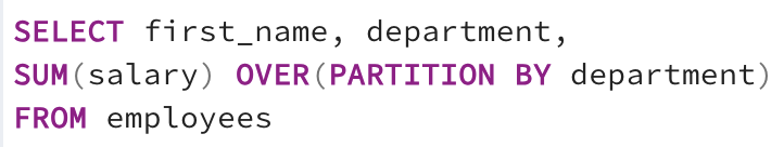
You could also use OVER() to show departmental salary in a column for each employee:
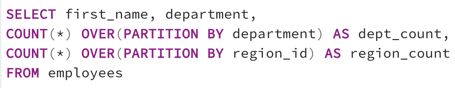
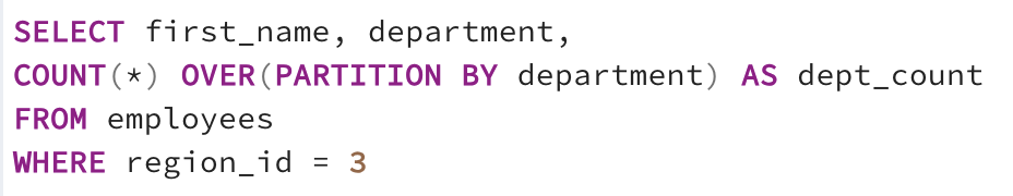
OVER() clause can be used more than once in a query. Here the departmental headcount and region headcount are shown in columns for each employee:
Finally, you can use WHERE clauses. Note that the OVER() clause occurs last in the query. As a result, the dept_count below will correctly show the COUNT() for region_id 3, not the COUNT() for the company:
Ordering Data in Window Frames
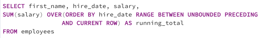
Show employee name, hire date, salary, and a running total of employee salaries ordered by hire date:
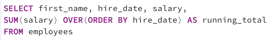
A more simple way to write this. Note that the RANGE BETWEEN UNBOUNDED PRECEDING AND CURRENT ROW is assumed:
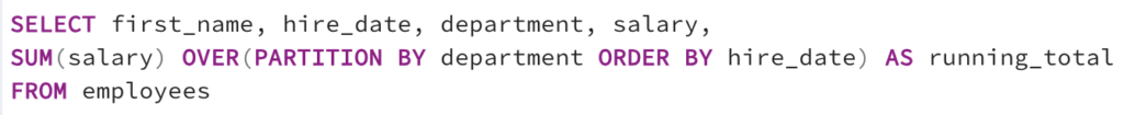
Show employee name, hire date, department, salary, and a running total of departmental salary. Note that the sum resets when a new department is reached in the table:
Show employee name, hire date, department, salary, and the sum of the salaries of the current and preceding employees:

Another way to show employee name, hire date, salary, and a running total of all 1000 employee salaries ordered by hire date:
RANK, FIRST_VALUE and NTILE Functions
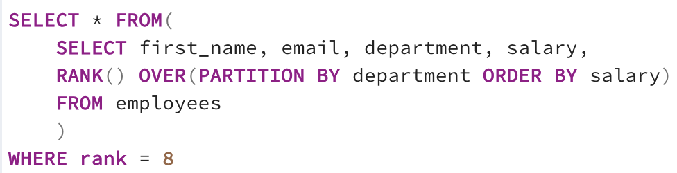
RANK() adds a column named rank that gives a numerical rank (1, 2, 3…) to the rows of the table, in the order that the table appears. In the case below, rows are partitioned by department, then ordered by salary. Note that the rank resets to “1” after each department:

Show only those people who are ranked 8th in their department:
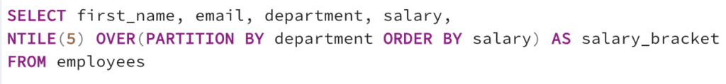
Rows in a table can be grouped into buckets, and these group numbers appear in a new column, Below, each department is grouped into 5 salary brackets:
FIRST_VALUE() will repeat the value of the first employee’s salary for every employee in the department. In this case, the lowest salary in each department will be included as a new column of data:

NTH_VALUE() will repeat the value of the nth employee’s salary for every employee in the department, starting with the nth employee. Employees before the nth value have a value of NULL in this column:

Working with LEAD and LAG Functions
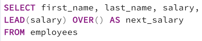
LEAD() allows a value from the next row to be used. Here, a column is created that lists the next employee’s salary:
LAG() allows a value from the previous row to be used. Here, a column is created that lists the previous employee’s salary:

LAG() can be used to show the next highest salary for a given row:

LAG() can also be used to show the next highest salary by department:

Working with Rollups and Cubes
This is the table “sales” we will be using for this section:

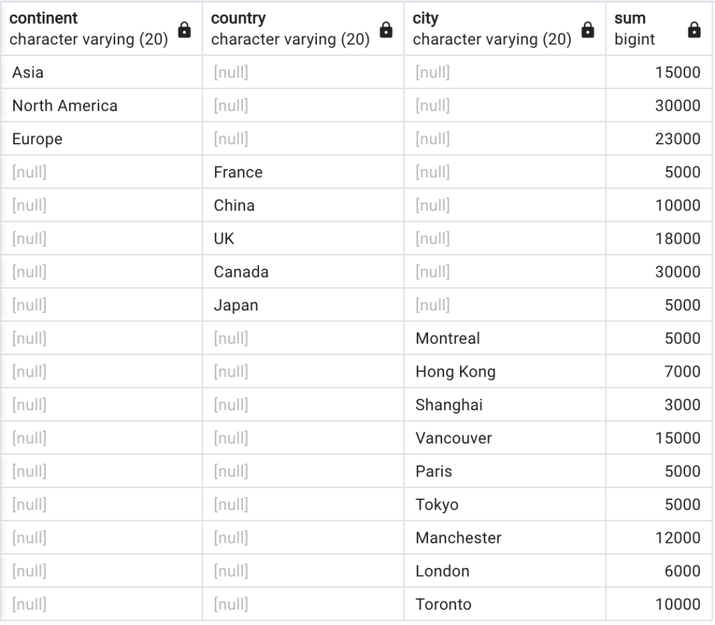
If we want to see units sold for continents, countries, and cities in one table, we can use the GROUP BY GROUPING SETS clause:
This is the resulting table:
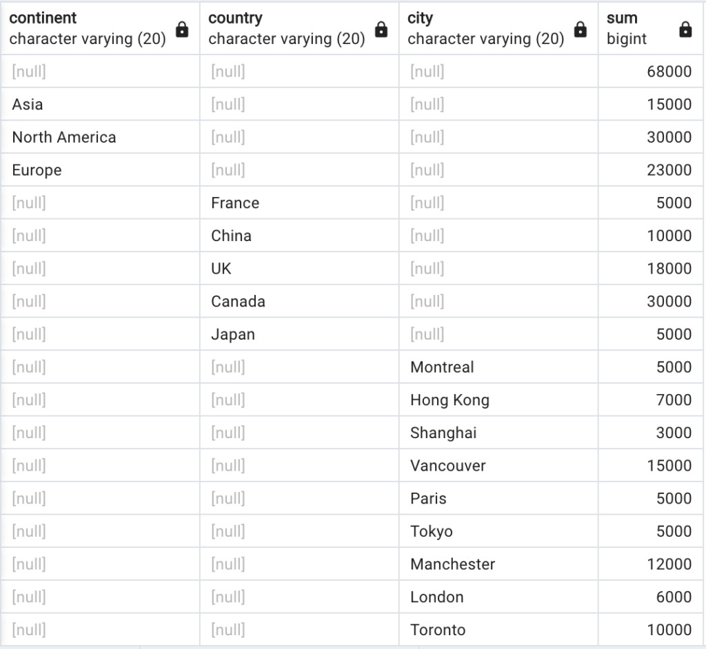
We can also include a line that shows the total units sold by adding ():

This is the resulting table:
Finally, we can perform a ROLLUP(). This shows units sold for every possible combination of groups. Some of this information ends up being redundant, but the table is still very useful:
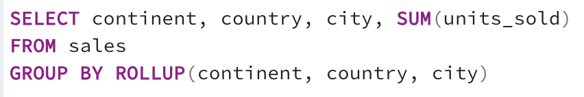
This is the resulting table:

Difficult Query Challenges
These exercises will use the tables: students, student_enrollment, courses, professors and teach.
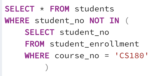
Write a query that finds students who do not take CS180. HINT: Make sure to consider students who are not enrolled in classes:
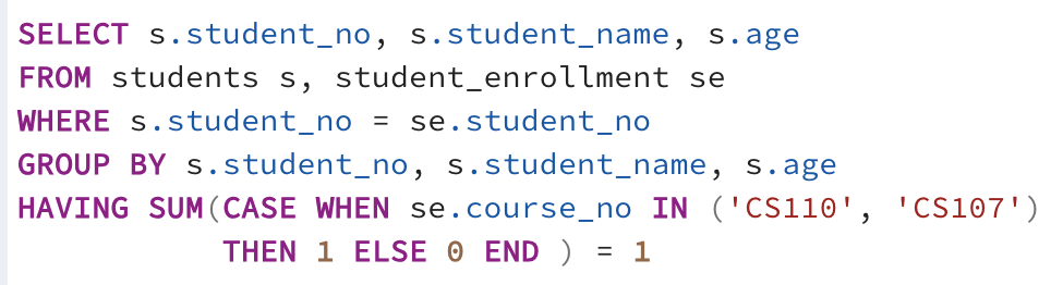
Write a query to find students who take CS110 or CS107 but not both:

Here is another solution to this problem:
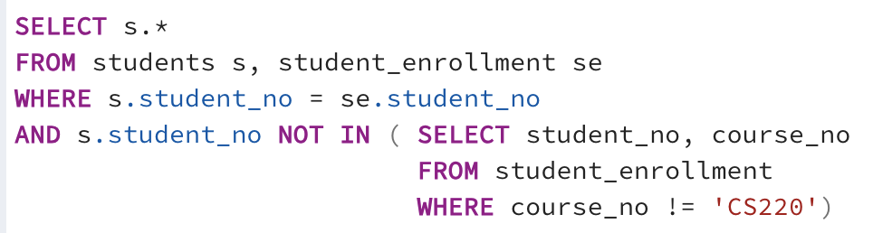
Write a query to find students who take CS220 and no other courses:
Write a query that finds those students who take at most 2 courses. Your query should exclude students that don’t take any courses as well as those that take more than 2 course.
Write a query to find students who are older than at most two other students: