Probability Distributions

Fundamentals of Probability Distribution

 A distribution shows the possible values a random variable can take and how frequently they occur.

Notation

Y = the actual outcome of an event.

y = One of the possible outcomes.

The probability of achieving an outcome y is:

or simply:

Since p(y) expresses the probability for each distinct outcome, we call p(y) the probability function.

Probability Distribution

A probability distribution is a statistical function that describes the probability of occurrence for each possible value of a discrete random variable. It provides a systematic way of assigning probabilities to the different outcomes or values of a random variable.

A probability frequency distribution consists of two components:

1. Values of the Random Variable: It lists all possible values that the random variable can take. For example, if we have a random variable representing the outcome of rolling a fair six-sided die, the possible values would be {1, 2, 3, 4, 5, 6}.
2. Probabilities: It assigns a probability to each possible value. The probabilities assigned must satisfy the following conditions:
   • Each probability is a non-negative value between 0 and 1.
   • The sum of all probabilities is equal to 1.

The probability distribution can be presented in various ways, depending on the context and the nature of the random variable. Common representations include tables, graphs, or mathematical formulas.

Record the frequency for each unique value, and divide it by the total number of elements.

Distribution Characteristics

mean – average value of the data. This is denoted µ.

variance – how spread out the data is. This is denoted σ².

Population Data vs. Sample Data

Population Data – all of the data.

Sample Data – just a part of the data.

Sample Data uses different notation for mean and variance. It is as follows:

Sample Mean – is denoted as x̄.

Sample Variance – is denoted as s².

Standard Deviation

Often, Standard Deviation is used instead of variance. For Populations, it is denoted by:

For Samples, Standard Deviation is simple denoted s.

Relationship Between Mean and Variance

A constant relationship between mean and variance exists for any distribution. ‘E(Y²)’ is read as ‘the expected value of Y²‘.

Types of Probability Distributions

Discrete Distributions – finite number of outcomes, like rolling a die or pulling a playing card. The equations we have covered so far apply to Discrete Distributions.

Continuous Distributions – infinite many outcomes, like recording time and distance. These use different formulas than the ones we have learned so far.

Notation Example

where:

• X = variable
• N = the type of distribution
• (µ, σ²) – the characteristics of the dataset (these can vary depending on the type of distribution)

Discrete Distributions

1. Equiprobable – all outcomes are equally likely. These follow a Uniform Distribution.
2. True or False outcomes – follow a Bernoulli Distribution.
3. Many Iterations – There are two outcomes per iteration. Follows a Binomial Distribution.
4. Unusual – Use the Poisson Distribution to test out how unusual an event frequency is for a given interval.

Continuous Distributions

1. Normal Distribution – often observed in nature.
2. Student’s-T Distribution – a small sample approximation of a Normal Distribution. This distribution handles extreme values significantly better.
3. Chi Squared Distribution – Asymmetric. Only consists of non-negative values. Does not often mirror real-life events. Used in Hypothesis Testing. Is used to test goodness of fit.
4. Exponential Distribution – useful when events are rapidly changing early on.
5. Logistic Distribution – useful in forecast analysis. Useful for determining a cutoff point for a successful analysis.

Characteristics of Discrete Distributions

• Finitely many distinct outcomes.
• Every unique outcome has a probability assigned to it.

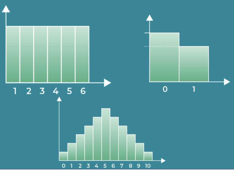
The Uniform Distribution

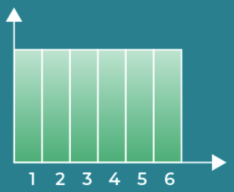
• All outcomes have equal probability, like a dice roll or a playing card draw.
• Note that the Expected Value of uniform distributions provide us with no information.
• Also, the mean and variance are uninterpretable.
• Uniform distributions are notated like this:

• The following is read as ‘variable X follows a discrete uniform distribution ranging from 3 to 7’.

Bernoulli Distribution

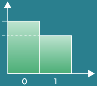
• This is used when there is one trial and two possible outcomes. Examples include a coin flip, a True/False question, or voting D or R in an election.
• Usually the probability (p) of at least one event is known, or past data indicating some experimental probability is known.
• Note that if the probability of one outcome is p, then the probability of the other outcome is p – 1.
• We usually select p such that p < 1 – p.
• We also typically assign a 0 or 1 to each outcome. Usually p is associated with the outcome 1, and p – 1 is associated with the outcome 0.
• Bernoulli Distributions are notated as below. The following is read ‘variable X follows a Bernoulli distribution with a probability of success equal to p’.

• The variance of Bernoulli events is always as noted below, but it brings us little value.

Binomial Distribution

• A Binomial Distribution can be thought of as a sequence of identical Bernoulli events.
• Notation below. n = the number of trials. p= the probability of an individual event succeeding.

• The following can be read as ‘the variable X has a binomial distribution with 10 trials and a likelihood of 0.6 to succeed on each individual trial’.

Bernoulli vs Binomial Distribution

• The Expected Value of a Bernoulli event E(Bernoulli event) suggests which outcome we expect for a single trial.
• The Expected Value of a Binomial Event E(Binomial Event) would suggest the number of times we expect to get a specific outcome.

The Probability Function p(y) in Binomial Distributions

• Probability Function – the likelihood of getting a given outcome a precise number of times.
• P(desired outcome) = p
• P(alternative outcome) = 1 – p
• The Probability Function for Binomial Distributions is below. Note that the n over y in parenthesis can ben thought of as ‘the number of Combinations of picking y many elements out of the total n’.

Example: GM stock has a 0.6 probability of going up on any given day. What is the probability of GM stock going up 3 days in a week? Here, n = 5, and p = 3.

The Expected Value in Binomial Distributions

If Y has a binomial distribution:

then the Expected Value of Y is:

Note that the above equation is identical to the formula for computing the Expected Values of Categorical Variables.

Variance and Standard Deviation in Binomial Distributions

Poisson Distributions

The Poisson Distribution deals with the frequency with which an event occurs within a specific interval. It shows the number of occurrences of each outcome, and probability of each one.

We denote a Poisson Distribution like this:

The following can be stated as ‘variable Y follows a poisson distribution with λ = 4’.

Probability Function for Poisson Distributions

Expected Values, Mean, and Variance in Poisson Distributions

Characteristics of Continuous Distributions

1. Sample space is infinite.
2. We cannot record the frequency of each distinct value.
3. Cannot be represented in tables.
4. Can be represented on a graph.
5. The probability for any individual value equals 0. P(X) = 0

Probability Density Function (PDF)

• The probability density function (PDF) is a function that describes the likelihood of a continuous random variable taking on a specific value within a given range of values.
• The PDF function satisfies the following two properties:
  • Non-negativity: The PDF is always non-negative, that is, f(x) >= 0 for all x in the domain of the random variable.
  • Normalization: The area under the curve of the PDF over its entire domain is equal to 1, that is, ∫f(x)dx = 1, where the integral is taken over the entire domain of the random variable.
• In other words, the PDF function gives the probability density of the random variable at each point in its domain. The height of the curve at a particular value of x indicates the relative likelihood of that value occurring.

Cumulative Distribution Function (CDF)

• The Cumulative Distribution Function (CDF) describes the probability of a random variable being less than or equal to a particular value. In other words, it gives the cumulative probability distribution of a random variable.
• The CDF is denoted by the symbol F(x) and is defined as the integral of the PDF function f(x) from negative infinity to x, that is,
• F(x) = ∫_{-∞}^x f(t)dt
• where x is any real number in the domain of the random variable.
• The CDF function satisfies the following properties:
  • Non-decreasing: The CDF is a non-decreasing function, that is, F(x) ≤ F(y) for any x ≤ y.
  • Bounded: The CDF is bounded between 0 and 1, that is, 0 ≤ F(x) ≤ 1 for any x.
  • Right-continuous: The CDF is right-continuous, that is, lim_{y→x+} F(y) = F(x).
• The value of the CDF at a specific value of x gives the probability that the random variable is less than or equal to that value. It can be used to calculate probabilities of events such as P(a ≤ X ≤ b), where a and b are any two real numbers in the domain of the random variable.
• In summary, the CDF is a fundamental concept in probability theory that provides a way to describe the probability distribution of a random variable in terms of the cumulative probabilities of the values it can take.

This function encompasses everything up to a certain value. We denote this F(y) for any continuous random variable y.

Note from the example graph that:

Probability of Intervals

Where a and b are points on a density curve, p(b > x > a) can be found by:

CDF vs PDF

Use Integrals to go from PDF to CDF:

Use Derivatives to go from CDF to PDF:

Expected Value and Variance

The Normal Distribution

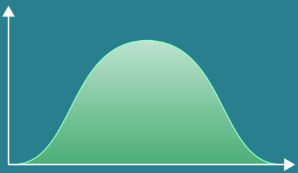
• Also known as the Gaussian Distribution or the Bell Curve.
• The Normal Distribution often appears in nature.
• Bell shaped and symmetrical.
• Most data occurs around the mean.
• Symmetrical wrt the mean. No skew.
• mean = median = mode

It is notated like this:

‘Variable X follows a Normal Distribution’:

PDF for Normal Distributions

Expected Value and Variance for Normal Distributions

σ² is usually given. If it is not, we can use this equation to calculate Variance of X:

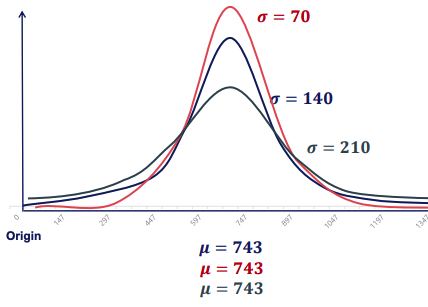
• Changing standard deviation changes the shape of the distribution.
• Small values of σ result in more data in the middle and thinner tails.
• Large values of σ result in less data in the middle and fatter tails.

The 68, 95, 99.7 Law

For any normally distributed event:

• 68% of all outcomes fall within 1 standard deviation away from the mean.
• 95% of all outcomes fall within 2 standard deviations of the mean.
• 99.7% of all outcomes fall within 3 standard deviations of the mean.

The Standard Normal Distribution

Transformation – A way in which we can alter every element of a distribution to get a new distribution.

You can add, subtract, divide, or multiple a distribution without changing the type of the distribution.

Addition moves the graph to the right.

Subtraction moves the graph to the left.

Multiplication shrinks the graph horizontally for values greater than one, and widens the graph for values less than one.

Division widens the graph horizontally for values greater than one, and shrinks the graph for values less than one.

Standardizing is a special kind of Transformation where we set E(X) = 0, and Var(X) = 1. Applying this to a Normal Distribution results in a Standard Normal Distribution.

Standardizing

We wish to move the graph to the left or right so that the mean (µ) is zero. To do this, subtract µ from every element:

Now we need to make the standard deviation (σ) equal to 1. To do this, we divide every element by σ:

Notation for Standard Normal Distributions:

Student’s T Distribution

• Remember that the Student’s T Distribution is a small sample size approximation of a Normal Distribution.
• Frequently used when conducting statistical analysis.
• Used in Hypothesis Testing with limited data.
• CDF table (T-table) ?

Notation

The Student’s T Distribution is notated as below, where k is degrees of freedom:

‘Variable Y follows a Student’s T Distribution with 3 degrees of freedom’:

Expected Value and Variance for Student’s T Distribution

If k > 2:

The Chi-Squared Distribution

• Chi-Squared Distributions are not usually seen in real life.
• They are used in Statistical Analysis for:
  • Hypothesis Testing
  • Computing confidence intervals
• Used when determining goodness of fit of categorical values.
• Asymmetric distribution.
• Mean can be found at the high point of the graph.

Notation

The Chi-Squared Distribution is notated as below, where k is degrees of freedom:

‘Variable Y follows a Chi-Squared Distribution with 3 degrees of freedom’:

Other Chi-Squared Equations

Chi-Squared Expected Value and Variance

A table of known values exist for this distribution.

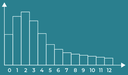
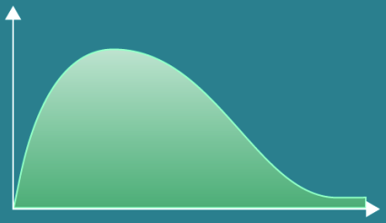
The Exponential Distribution

• Starts off high.
• Initially decreases.
• Eventually plateuing
• Example: views of a popular YouTube video.
  • Agregate amount of views keeps increasing.
  • Number of new ones diminishes.

Notation

The Exponential Distribution is notated as below, where λ is the scale or rate parameter.:

‘Variable X follows an Exponential Distribution with a scale of 1/2’:

Rate Parameter (λ)

The Rate Parameter (λ) determines:

1. How fast the CDF/PDF curve reaches the point of plateauing.
2. How spread out the graph is.

Expected Value and Variance for the Exponential Distribution

Unlike the Standard and Chi-Squared Distributions, there is no table of known variables.

A Common Transformation

If we take the natural logarithm of every set of an exponential distribution, and get a normal distribution. Then, we can run linear regressions.

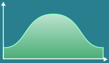
The Logistic Distribution

• Used when trying to determine how continuous variable inputs can affect the probability of a binary outcome, such as sports forecasting.
• The mean determines where the graph will be centered. The location or scale parameter determines how spread out the graph is.

Notation

The Logistic Distribution is notated as below, where S is the scale parameter. Note that the mean (µ) is also known as the Location:

‘Variable Y follows a Logistic Distribution with location 6, and a scale of 3’:

Expected Value and Variance

Probability Distribution Cheat Sheet